Summary

If you do not want to read through the entire article:

Based on the simulations presented, in my opinion, the best way to handle errors calculated from replicates of experiments which involve fitting the data is the following:

• Fit the data from each replicate independently.
• Take the mean of the estimates for the fitted values (here - k values, \(\bar{k}\)) obtained from each fit.
• Calculate the standard error of the mean for \(\bar{k} \;\) (\(SEM(\bar{k})\)).
• Propagate the standard error of fit to arrive at a fitting error for \(\bar{k} \;\) (\(\sigma_{fit}(\bar{k})\)).
• Combine the errors by squaring them, summing them and taking the square root (\(\sigma_{tot}(\bar{k}) = \sqrt{(\sigma_{fit}(\bar{k}))^2 + (SEM(\bar{k}))^2}\)), thus arriving at a final value for k with quantified uncertainty (\(\bar{k} \pm \sigma_{tot}(\bar{k})\)).

The presented simulations show that a random effects model also is also effective. However, for the vast majority of chemists/wet lab scientists (?) interested in appropriately accounting for error as assessed by repeated measurements, the above workflow should be sufficient in the majority of cases.

The Problem

You have a chemical reaction of the following type:

\(A \longrightarrow B\)

With a rate law:

\(\frac{\partial[A]}{dt} = -k[A]\)

You are interested in calculating the rate constant of the reaction so that you can compare the experimental and DFT-calculated barriers for the reaction (\(\Delta G^{\ddagger}_{A \rightarrow B}\)).¹

You remember from your old undergrad textbook that you can determine the rate constant through a simple linear regression:

\(ln([A]) = -kt + ln[A]_0\)

However, you also read that you should measure several datasets for the kinetics so that you can quantify the error associated with \(\Delta G^{\ddagger}_{A \rightarrow B}\). Being a diligent scientist you had read that n = 3 systematically severely underestimates standard deviation, so you decided to monitor ten independent samples over time (five would have also been acceptable, but you are early in your PhD and you have time), so you measured 10 repeats of your reaction over time. Let’s generate ten datasets that look approximately like what you would expect:

library(dplyr)
library(ggplot2)

# Function for simulating data
synth_dat_fn <- function(replicates,sd_k,
                         sd_A0,t_samp,noise,seed){
  # Sample k
  set.seed(seed)
  ks <- rnorm(replicates, 1e-3, sd_k)
  i <- 1
  out_df <- data.frame(repl = c(),
                       t = c(),
                       Conc_A_M = c())
  
  # Generate data for each sampled k
  for (k in ks){
    A0 <- rnorm(1,0.05,sd_A0)
    
    loop_df <- data.frame(repl = i,
                          t = seq(0,2000,by = t_samp)) %>%
      mutate(noise = rnorm(length(t),0,noise),
             Conc_A_M = exp(log(A0) - k*t) + noise)
    
    out_df <- rbind(out_df,
                    loop_df)
    
    i <- i + 1
  }
  
  return(out_df)
}

# Generate the data
kin_df <- synth_dat_fn(10,5e-5,
                       5e-3,100,5e-4,1)

print(head(kin_df))
##   repl   t         noise   Conc_A_M
## 1    1   0  1.949216e-04 0.05775383
## 2    1 100 -3.106203e-04 0.05193422
## 3    1 200 -1.107350e-03 0.04631404
## 4    1 300  5.624655e-04 0.04360573
## 5    1 400 -2.246680e-05 0.03904687
## 6    1 500 -8.095132e-06 0.03545421

# Plot the data
dat_plot <- ggplot(data = kin_df,
                   aes(x = t,
                       y = Conc_A_M,
                       color = as.factor(repl))) +
  geom_point() +
  theme_classic() +
  labs(x = "Time (s)",
       y = "[A] (M)") +
  theme(legend.position = "none")

print(dat_plot)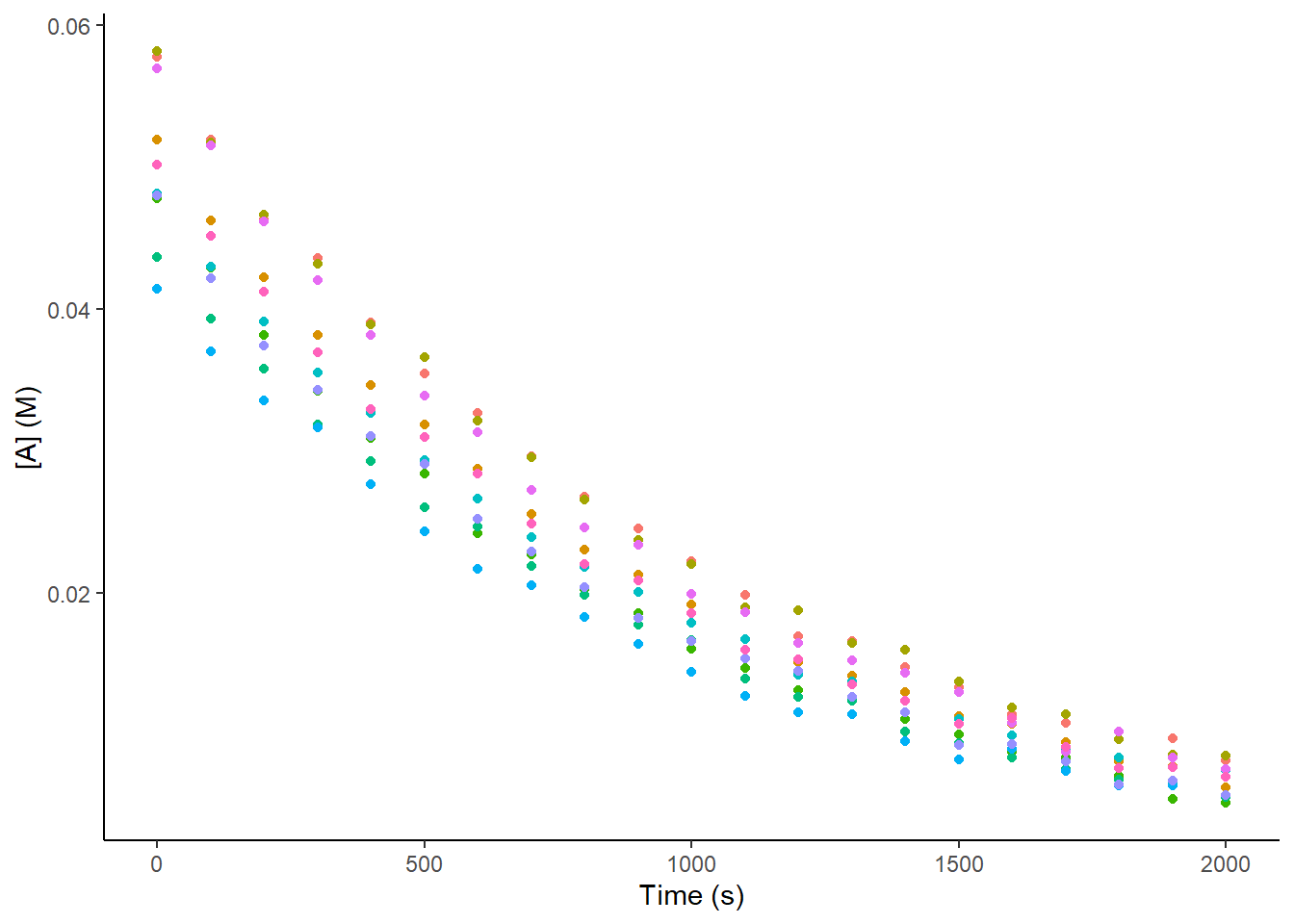

But what do you do now? Do you average all your data and perform linear regression on these averages? But if you do that, how do you account for the standard deviation that these averages have? The linear regression does not account for this deviation, as you have not indicated this anywhere in your fitting process.

This article will explain what to do, illustrate how with R code² and explain why by way of using synthetic data.

Simulations

There are several approaches that I have seen people reach for when confronted with this problem. In order to illustrate how each one performs, some ground-truth to compare to is required.

Let’s use the data simulated above - it comes from sampling 10 random values of k from a normal distribution with a mean of \(10^{-3} s^{-1}\) and a standard deviation of \(5 \cdot 10^{-5} s^{-1}\). This means that the ground truth corresponds to a value of \(k_{Ground \; Truth} = 10^{-3} \pm 1.6 \cdot 10^{-5} s^{-1}\) where the error expressed is the standard error (of the mean - calculated as standard deviation divided by square root of sample size).

Because some Gaussian noise was added to the datapoints generated from each unique value of k, the methods will not return exactly this value, but they should be able to get closer the smaller we make the noise. This noise of measurement will be reflected in the standard error of the fit.³

library(tidyr)

# Function to generate data at different noise levels
noise_lvl_fn <- function(noise_list){
  # Generate empty df with same columns
  out_df <- synth_dat_fn(10,5e-5,
                         5e-3,100,5e-4,1) %>%
    mutate(noise_lvl = "none") %>%
    filter(repl == 100)
  
  i <- 0
  
  n_dat <- seq(10,100,by = 10)
  
  # Loop through levels of noise and no of datapoints
  for (noise_lvl in noise_list){
    i <- i + 1
    for (n in n_dat) {
      loop_df <- synth_dat_fn(10,5e-5,
                              5e-3,n,noise_lvl,n+i) %>%
        mutate(noise_lvl = i,
               data_density = -2/log10(1/n) - 1)
      
      
      out_df <- rbind(out_df,
                      loop_df)
    }
  }
  
  out_df <- out_df
  
  return(out_df)
}

# Generate the data and get means and sds
noise_lvls <- noise_lvl_fn(c(1e-5,0.001,0.005,
                             0.01,0.02,0.05)) %>%
  group_by(repl,noise_lvl,data_density) %>%
  mutate(fit_k = lm(log(Conc_A_M) ~ t)$coef[[2]],
         SE_k = summary(lm(
           log(Conc_A_M) ~ t))$coefficients[2,2]) 

noise_min_df <- noise_lvls %>%
                ungroup(repl) %>%
                slice_head() %>%
                mutate(mean_fit_k = abs(mean(fit_k)),
                mean_SE_k = mean(SE_k),
                upr_k = mean_fit_k + mean_SE_k,
                lwr_k = mean_fit_k - mean_SE_k)

# Plot the data
noise_plot <- ggplot(data = noise_min_df,
                     aes(color = data_density,
                         x = mean_fit_k)) +
  geom_point(aes(y = mean_SE_k),
             size = 3) +
  geom_vline(xintercept = 1e-3,
             linewidth = 0.7,
             alpha = 0.3,
             linetype = 2,
             color = "red") +
  annotate("text",
           x = 1.2e-3, y = 7e-4,
           label = "Ground \n Truth",
           color = "red",
           size = 3) +
  labs(x = "Mean value of k (n = 10)",
       y = "Mean SE of k (n = 10)",
       color = "Data density") +
  scale_color_continuous(high = "#132B43", 
                        low = "#56B1F7") +
  facet_wrap(~ factor(noise_lvl)) +
  theme_classic() +
  theme(legend.position = "bottom")

print(noise_plot)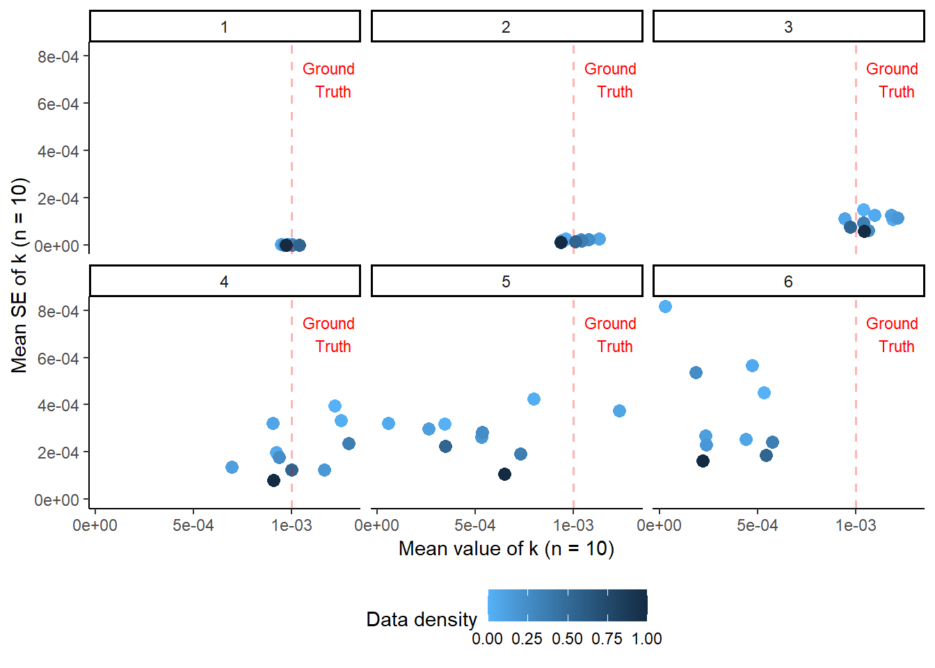

This illustrates how low noise measurements can achieve results comparable to those of higher noise measurements with fewer datapoints. Therefore, one of the first considerations when planning kinetic measurements is “How much measurement error does my chosen method inherently have?”. In cases such as NMR, the error is relatively small, whereas in something like HPLC (which also requires calibration curves) it may be larger, especially if sample preparation is complex (e.g. many filtration & dilution steps). The more noise a measurement has, the more timepoints you should collect, which will minimize the contribution of the error arising from fitting the model.

Now let’s test some of the common methods scientists reach for when confronted with this problem.

Method 1 - Fit on the average values

A very common approach to this problem is to average the observations at a given timepoint, fit the equation and report the error arising from the fit as the error for k. This does not take into account the deviation of the means, leading to an incorrect answer. To illustrate this, below are two datasets which have similar means for the timepoints and therefore similar mean k values, but while the ground truth error associated with k is the same, the obtained error for the fit is vastly different:

library(patchwork)

# Filter for low and high noise and take means across replicates
means_df <- noise_lvls %>%
  filter(noise_lvl %in% c(1,3) & data_density == 0) %>%
  group_by(noise_lvl,t) %>%
  mutate(mean_A = mean(Conc_A_M),
         sd_A = sd(Conc_A_M),
         upr_A = mean_A + sd_A,
         lwr_A = mean_A - sd_A) %>%
  filter(repl == 1) %>%
  ungroup()

# Check the fit for each
# low noise
print(summary(lm(log(Conc_A_M) ~ t, 
                 data = means_df %>%
                   filter(noise_lvl == 1))))
## 
## Call:
## lm(formula = log(Conc_A_M) ~ t, data = means_df %>% filter(noise_lvl == 
##     1))
## 
## Residuals:
##        Min         1Q     Median         3Q        Max 
## -0.0011768 -0.0001697  0.0001469  0.0002638  0.0008297 
## 
## Coefficients:
##               Estimate Std. Error t value Pr(>|t|)    
## (Intercept) -2.945e+00  2.113e-04  -13933   <2e-16 ***
## t           -9.834e-04  1.808e-07   -5440   <2e-16 ***
## ---
## Signif. codes:  0 '***' 0.001 '**' 0.01 '*' 0.05 '.' 0.1 ' ' 1
## 
## Residual standard error: 0.0005017 on 19 degrees of freedom
## Multiple R-squared:      1,	Adjusted R-squared:      1 
## F-statistic: 2.959e+07 on 1 and 19 DF,  p-value: < 2.2e-16

# High noise
print(summary(lm(log(Conc_A_M) ~ t, 
                 data = means_df %>%
                   filter(noise_lvl == 3))))
## 
## Call:
## lm(formula = log(Conc_A_M) ~ t, data = means_df %>% filter(noise_lvl == 
##     3))
## 
## Residuals:
##      Min       1Q   Median       3Q      Max 
## -1.11529 -0.06730  0.01909  0.23786  0.55043 
## 
## Coefficients:
##               Estimate Std. Error t value Pr(>|t|)    
## (Intercept) -3.0432069  0.1746454 -17.425 3.84e-13 ***
## t           -0.0010392  0.0001494  -6.956 1.25e-06 ***
## ---
## Signif. codes:  0 '***' 0.001 '**' 0.01 '*' 0.05 '.' 0.1 ' ' 1
## 
## Residual standard error: 0.4145 on 19 degrees of freedom
## Multiple R-squared:  0.718,	Adjusted R-squared:  0.7032 
## F-statistic: 48.39 on 1 and 19 DF,  p-value: 1.252e-06

# Print the plots and combine side by side
means_plot <- function(df,log_y_n){
  if(log_y_n == T){
    # Create the log plot
    out_plot <- ggplot(data = df,
                       aes(x = t)) +
      geom_point(aes(y = log(mean_A)),
                 size = 3) +
      labs(y = "Mean ln([A]) (n = 10)",
           x = "Time (s)") +
      theme_classic()
  }
  else{
    # Create the plot without logs
    out_plot <- ggplot(data = df,
                       aes(x = t)) +
      geom_errorbar(aes(ymin = lwr_A,
                        ymax = upr_A),
                    width = 0.3) +
      geom_point(aes(y = mean_A),
                 size = 3) +
      labs(y = "Mean [A] (n = 10)",
           x = "Time (s)") +
      theme_classic()
  }
  
  return(out_plot)
}

# Generate combined plot
comb_plot <- means_plot(means_df %>%
                          filter(noise_lvl == 1),
                        F) +
  means_plot(means_df %>%
               filter(noise_lvl == 3),
             F) +
  means_plot(means_df %>%
               filter(noise_lvl == 1),
             T) +
  means_plot(means_df %>%
               filter(noise_lvl == 3),
             T) +
  plot_layout(nrow = 2, ncol = 2,
              axes = "collect")

print(comb_plot)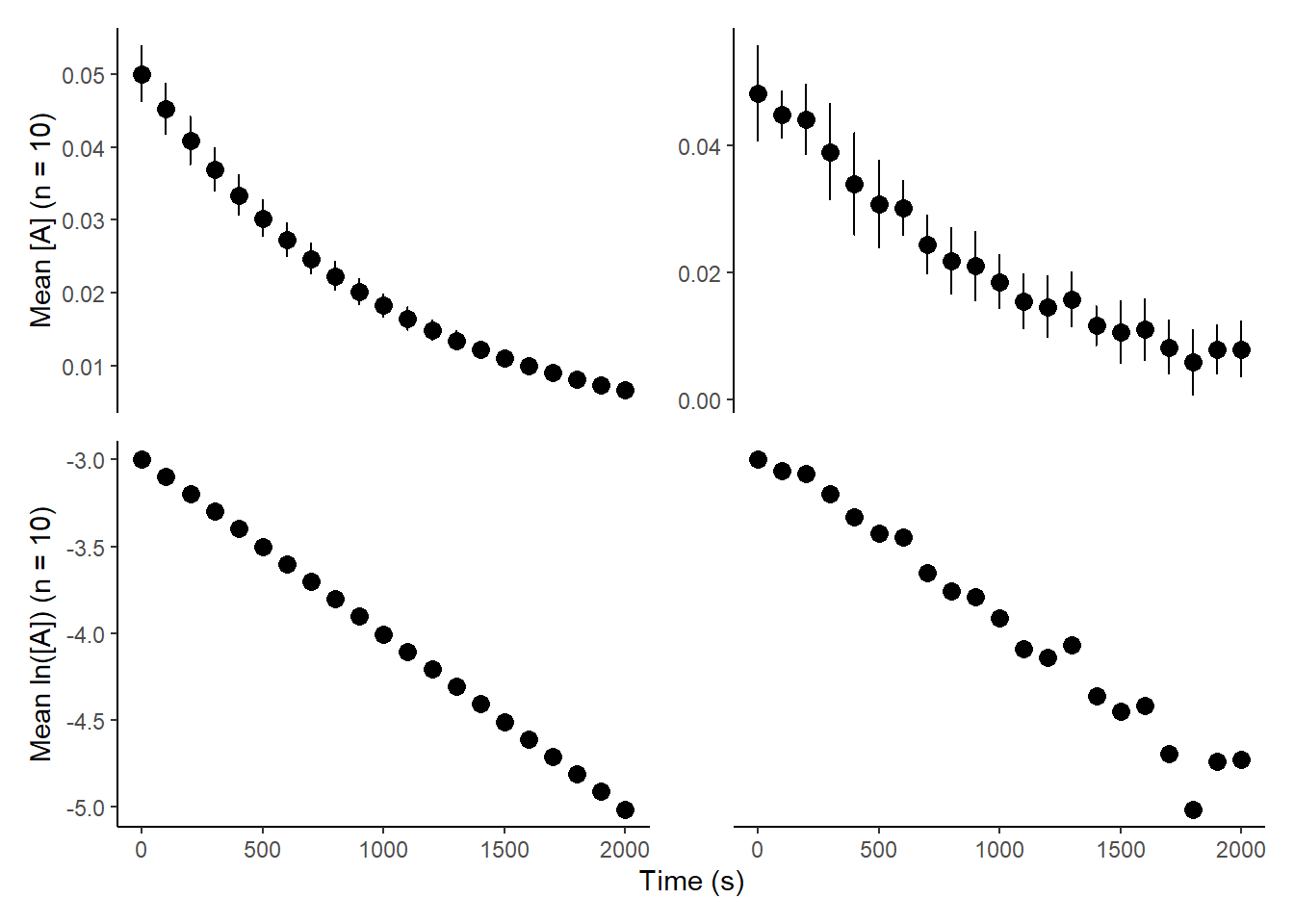

The two values for k we are provided are \(0.9 \cdot 10^{-3} \pm 1.8 \cdot 10^{-7} s^{-1}\) and \(1.0 \cdot 10^{-3} \pm 1.5 \cdot 10^{-4} s^{-1}\) - the k values are accurate, but the former error is too low by two orders of magnitude and the latter is one order of magnitude too large, despite fairly.

“You just need to propagate the standard deviation into the final value of k!”. Which standard deviation?⁴

Method 2 - Fit on all the values

Maybe we are overthinking this. Maybe we should just put all the data into the regression and take whatever value comes out.

# Evalute only for low noise
global_fit_df <- noise_lvls %>%
  filter(noise_lvl == 1 & data_density == 0) %>%
  mutate(Conc_A_M = Conc_A_M/max(Conc_A_M))

# Evaluate the model
print(summary(lm(log(Conc_A_M) ~ t, 
                 data = global_fit_df)))
## 
## Call:
## lm(formula = log(Conc_A_M) ~ t, data = global_fit_df)
## 
## Residuals:
##       Min        1Q    Median        3Q       Max 
## -0.093401 -0.017379 -0.000136  0.018552  0.090787 
## 
## Coefficients:
##               Estimate Std. Error  t value Pr(>|t|)    
## (Intercept)  1.357e-04  4.343e-03    0.031    0.975    
## t           -1.012e-03  3.715e-06 -272.468   <2e-16 ***
## ---
## Signif. codes:  0 '***' 0.001 '**' 0.01 '*' 0.05 '.' 0.1 ' ' 1
## 
## Residual standard error: 0.0326 on 208 degrees of freedom
## Multiple R-squared:  0.9972,	Adjusted R-squared:  0.9972 
## F-statistic: 7.424e+04 on 1 and 208 DF,  p-value: < 2.2e-16

# Show the fit
global_fit_plot <- ggplot(data = global_fit_df,
                          aes(y = log(Conc_A_M),
                              x = t)) +
  geom_point(aes(color = repl),
             size = 3) +
  geom_smooth(se = T,
              method = "lm") +
  labs(y = "Mean ln([A]) (n = 10)",
       x = "Time (s)") +
  theme_classic()

print(global_fit_plot)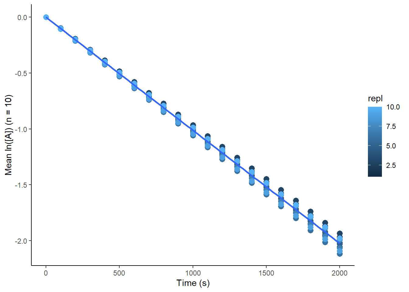

Using data with effectively no noise, this gives us a value of \(1.0 \cdot 10^{-3} \pm 3.72 \cdot 10^{-6} s^{-1}\) - k is accurate, but the error is underestimated. This is because we have treated the data as if we made 10 simultaneous measurements at each timepoint, rather than treating them as independent experiments.⁵

Method 3 - Fit independently and propagate

To treat these as separate experiments, they should be fit independently. Now if we take a mean and SEM of these 10 ks we obtained, we will obtain a mean k value and a SEM. But each of the 10 ks has an associated error which comes from the fit, how do we account for this? We must simply propagate this error. Now we have two error terms for \(\bar{k}\), the error from the fit that we propagated \(\sigma_{fit}(\bar{k})\) and the standard error of the mean from taking the means of the fitted ks \(SEM(\bar{k})\). To combine them, we sum their squares and take the square root:

# Fifth code block
ind_fit_df <- noise_lvls %>%
  group_by(repl,noise_lvl,data_density) %>%
  slice_head() %>%
  ungroup(repl) %>%
  dplyr::select(c(fit_k,SE_k,noise_lvl)) %>%
  mutate(mean_k = mean(abs(fit_k)),
         sem_k_repl = sd(abs(fit_k))/sqrt(10),
         sem_k_fit = sqrt(sum(SE_k^2)/10),
         sem_k_tot = sqrt(sem_k_fit^2 + sem_k_repl^2)) %>%
  slice_head()

# Plot the values of error
error_plot <- ggplot(data = ind_fit_df,
                     aes(x = factor(noise_lvl),
                         y = sem_k_tot,
                         color = data_density)) +
  geom_point(size = 3) +
  geom_hline(yintercept = 5e-05/sqrt(10),
             linewidth = 0.7,
             alpha = 0.3,
             linetype = 2,
             color = "red") +
  annotate("text",
           y = 4e-5, x = factor(5),
           label = "Ground Truth",
           color = "red",
           size = 5) +
  labs(x = "Mean value of k (n = 10)",
       y = "Mean SEM of k (n = 10)",
       color = "Data density") +
  scale_color_continuous(high = "#132B43", 
                         low = "#56B1F7") +
  theme_classic() +
  theme(legend.position = "bottom")

print(error_plot)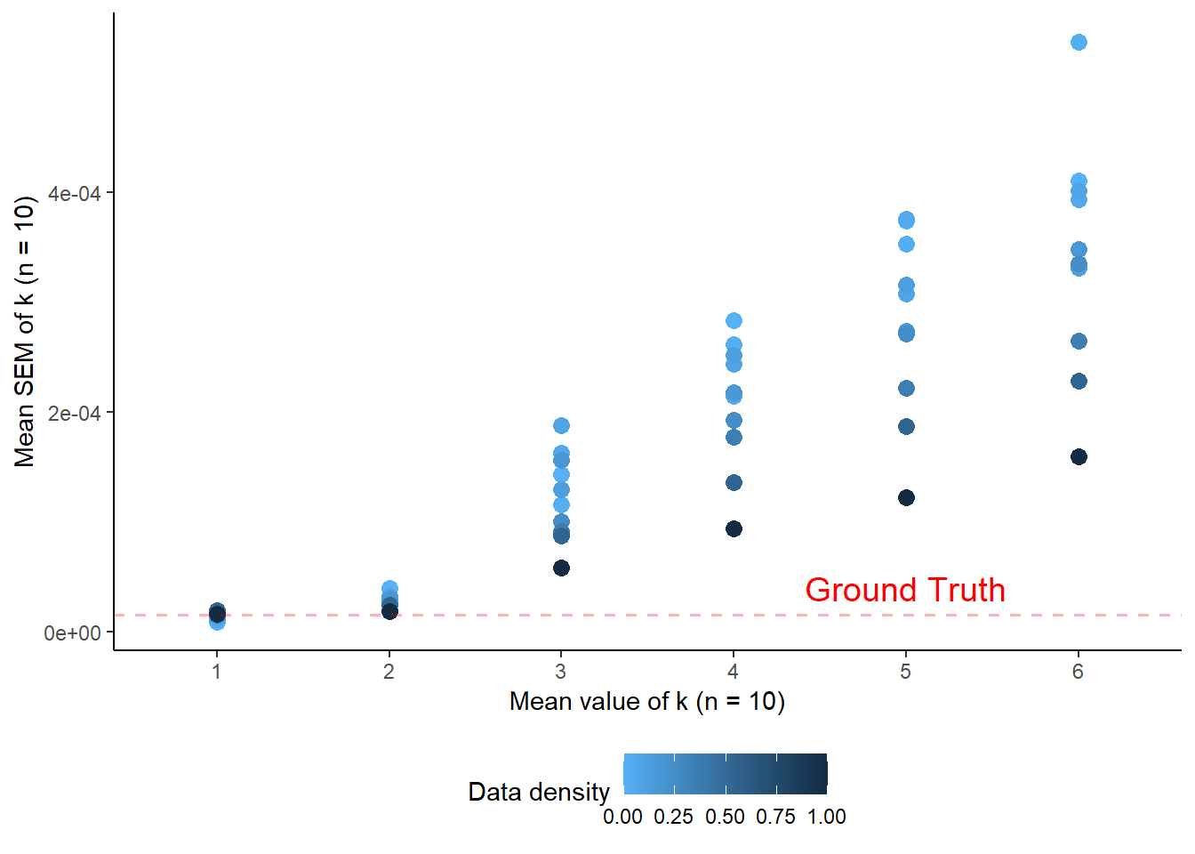

The plot clearly shows that when very little noise is present, the SEM is correctly estimated to be the same as the ground truth SEM from the simulated data, indicating that this is indeed the correct approach. It also shows that as noise increases, the amount of datapoints collected becomes more important, as expected.

Method 4 - Random effects modeling

I will admit, I have never met a chemist who treated this problem using random effects modeling. However, I was curious how it would fare. Here each replicate is treated as a categorical variable, sampled from a distribution of values, and both intercept and slope for each replicate is allowed to vary. You will notice that this seems very similar to treating individual fits, but the errors are handled by the package in this case!

library(lme4)

# Get the df ready
rand_eff_df <- noise_lvls %>%
  filter(data_density == 0) %>%
  group_by(noise_lvl) %>%
  group_split()

# Function to apply random effects
# per noise level and get coefs +- error
rand_eff_fn <- function(df_list){
  # Empty df to write
  out_df <- data.frame(k = c(),
                       se_k = c(),
                       noise_lvl = c())
  
  for (i in seq(1,length(df_list),
                by = 1)) {
    rand_eff_mod <- lmer(log(Conc_A_M) ~ t + (t | repl),
                         data = df_list[[i]],
                         control = lmerControl(
                           optimizer ="Nelder_Mead"))
    
    loop_df <- data.frame(k = abs(summary(
                            rand_eff_mod)$coefficients[2,1]),
                          se_k = summary(
                            rand_eff_mod)$coefficients[2,2],
                          noise_lvl = i)
    
    out_df <- rbind(out_df,
                    loop_df)
  }
  
  return(out_df)
}

rand_eff_est <- rand_eff_fn(rand_eff_df)

print(rand_eff_est)
##              k         se_k noise_lvl
## 1 0.0010122836 9.250687e-06         1
## 2 0.0010386469 2.720185e-05         2
## 3 0.0010855084 5.669244e-05         3
## 4 0.0009998658 1.016175e-04         4
## 5 0.0004994944 1.185252e-04         5
## 6 0.0003595186 1.213749e-04         6

Interestingly, this approach is both more concise code-wise and more robust towards noise compared to the individual fits! Personally I will definitely give this a try if the need arises, but I understand that most chemists will not be using R.